10.1 What is Sorting?
Sorting is an algorithm that arranges the elements of a list in a certain order [either ascending or descending]. The output is a permutation or reordering of the input.
10.2 Why is Sorting Necessary?
Sorting is one of the important categories of algorithms in computer science and a lot of research has gone into this category. Sorting can significantly reduce the complexity of a problem, and is often used for database algorithms and searches.
10.3 Classification of Sorting
Algorithms Sorting algorithms are generally categorized based on the following parameters.
By Number of Comparisons
In this method, sorting algorithms are classified based on the number of comparisons. For comparison based sorting algorithms, best case behavior is O(nlogn) and worst case behavior is O(n 2 ). Comparison-based sorting algorithms evaluate the elements of the list by key comparison operation and need at least O(nlogn) comparisons for most inputs. Later in this chapter we will discuss a few non – comparison (linear) sorting algorithms like Counting sort, Bucket sort, Radix sort, etc. Linear Sorting algorithms impose few restrictions on the inputs to improve the complexity.
By Number of Swaps
In this method, sorting algorithms are categorized by the number of swaps (also called inversions).
By Memory Usage
Some sorting algorithms are “in place” and they need O(1) or O(logn) memory to create auxiliary locations for sorting the data temporarily.
By Recursion
Sorting algorithms are either recursive [quick sort] or non-recursive [selection sort, and insertion sort], and there are some algorithms which use both (merge sort).
By Stability
Sorting algorithm is stable if for all indices i and j such that the key A[i] equals key A[j], if record R[i] precedes record R[j] in the original file, record R[i] precedes record R[j] in the sorted list. Few sorting algorithms maintain the relative order of elements with equal keys (equivalent elements retain their relative positions even after sorting).
By Adaptability
With a few sorting algorithms, the complexity changes based on pre-sortedness [quick sort]: presortedness of the input affects the running time. Algorithms that take this into account are known to be adaptive.
10.4 Other Classifications Another method of classifying sorting algorithms is:
• Internal Sort
• External Sort
Internal Sort
Sort algorithms that use main memory exclusively during the sort are called internal sorting algorithms. This kind of algorithm assumes high-speed random access to all memory.
External Sort
Sorting algorithms that use external memory, such as tape or disk, during the sort come under this category.
10.5 Bubble Sort Bubble sort is the simplest sorting algorithm. It works by iterating the input array from the first element to the last, comparing each pair of elements and swapping them if needed. Bubble sort continues its iterations until no more swaps are needed. The algorithm gets its name from the way smaller elements “bubble” to the top of the list. Generally, insertion sort has better performance than bubble sort. Some researchers suggest that we should not teach bubble sort because of its simplicity and high time complexity.
The only significant advantage that bubble sort has over other implementations is that it can detect whether the input list is already sorted or not.
Implementation
void BubbleSort(int A[], int n) {
=
for (int pass n -1; pass >= 0; pass--){
for (int i = 0; i <= pass - 1; i++) if(A[i]> A[i+1]) { // swap elements
int temp = A[i]; A[i]-A[i+1]; A[i+1]=temp;
{
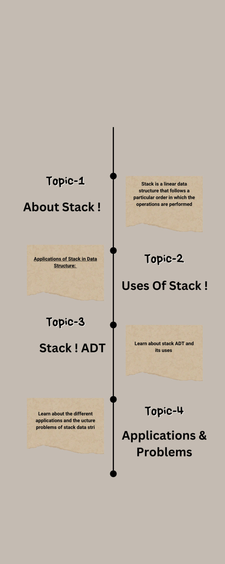
Algorithm takes O(n 2 ) (even in best case). We can improve it by using one extra flag. No more swaps indicate the completion of sorting. If the list is already sorted, we can use this flag to skip the remaining passes.
void BubbleSortImproved (int A[], int n) { int pass, i, temp, swapped = 1;
=
for (pass n -1; pass >= 0 && swapped; pass--) {
swapped = 0;
for (i=0;i<= pass - 1; i++) { if(A[i]> A[i+1]) {
// swap elements
temp =A[i]; A[i]-A[i+1]; A[i+1] = temp;
swapped = 1;
This modified version improves the best case of bubble sort to O(n). Performance
Performance
10.6 Selection Sort
Selection sort is an in-place sorting algorithm. Selection sort works well for small files. It is used for sorting the files with very large values and small keys. This is because selection is made based on keys and swaps are made only when required.
Advantages
• Easy to implement
• In-place sort (requires no additional storage space)
Disadvantages
• Doesn’t scale well: O(n 2 )
Algorithm
1. Find the minimum value in the list
2. Swap it with the value in the current position
3. Repeat this process for all the elements until the entire array is sorted
This algorithm is called selection sort since it repeatedly selects the smallest element.
Implementation
void Selection(int A [], int n) { int i, j, min, temp;
for (i=0; i<n-1; i++) { mini;
}
for (j=i+1;j< n; j++){ if(A [i] < A [min])
min = j;
// swap elements
temp-A[min]; A[min] =A[i]; A[i] = temp;
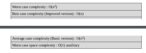
Performance
10.7 Insertion Sort Insertion sort is a simple and efficient comparison sort. In this algorithm, each iteration removes an element from the input data and inserts it into the correct position in the list being sorted. The choice of the element being removed from the input is random and this process is repeated until all input elements have gone through.
Advantages
• Simple implementation
• Efficient for small data
• Adaptive: If the input list is presorted [may not be completely] then insertions sort takes O(n + d), where d is the number of inversions
• Practically more efficient than selection and bubble sorts, even though all of them have O(n 2 ) worst case complexity
• Stable: Maintains relative order of input data if the keys are same
• In-place: It requires only a constant amount O(1) of additional memory space
• Online: Insertion sort can sort the list as it receives it
Algorithm
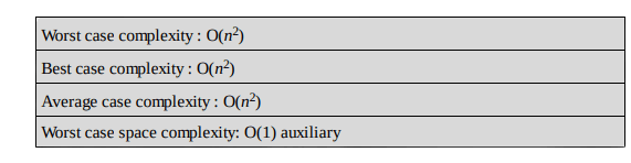
Every repetition of insertion sort removes an element from the input data, and inserts it into the correct position in the already-sorted list until no input elements remain. Sorting is typically done in-place. The resulting array after k iterations has the property where the first k + 1 entries are sorted.
Each element greater than x is copied to the right as it is compared against x.
Implementation
void InsertionSort(int A[], int n) { int i, j, v;
for (i=1;i<=n-1; i++) { v = A[i];
j=i;
}
while (A[j-1]> v && j>= 1) {
A[j] = Aj-1];
j--;
Aj]=v;
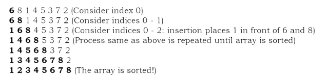
Example
Given an array: 6 8 1 4 5 3 7 2 and the goal is to put them in ascending order.
Analysis
Worst case analysis
Worst case occurs when for every i the inner loop has to move all elements A[1], . . . , A[i – 1] (which happens when A[i] = key is smaller than all of them), that takes Θ(i – 1) time

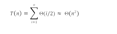
Average case analysis
For the average case, the inner loop will insert A[i] in the middle of A[1], . . . , A[i – 1]. This takes Θ(i/2) time.
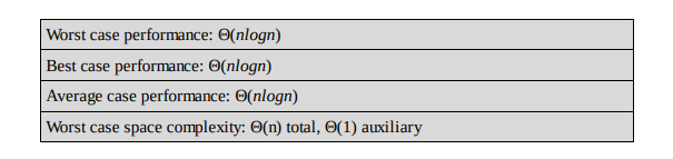
Performance
If every element is greater than or equal to every element to its left, the running time of insertion sort is Θ(n). This situation occurs if the array starts out already sorted, and so an already-sorted array is the best case for insertion sort.

Comparisons to Other Sorting Algorithms Insertion sort is one of the elementary sorting algorithms with O(n 2 ) worst-case time. Insertion sort is used when the data is nearly sorted (due to its adaptiveness) or when the input size is small (due to its low overhead). For these reasons and due to its stability, insertion sort is used as the recursive base case (when the problem size is small) for higher overhead divide-and-conquer sorting algorithms, such as merge sort or quick sort.
Notes
• Bubble sort takes comparisons and swaps (inversions) in both average case and in worst case.
• Selection sort takes comparisons and n swaps.
• Insertion sort takes comparisons and swaps in average case and in the worst case they are double.
• Insertion sort is almost linear for partially sorted input.
• Selection sort is best suits for elements with bigger values and small keys
10.8 Shell Sort
Shell sort (also called diminishing increment sort) was invented by Donald Shell. This sorting algorithm is a generalization of insertion sort. Insertion sort works efficiently on input that is already almost sorted. Shell sort is also known as n-gap insertion sort. Instead of comparing only the adjacent pair, shell sort makes several passes and uses various gaps between adjacent elements (ending with the gap of 1 or classical insertion sort).
In insertion sort, comparisons are made between the adjacent elements. At most 1 inversion is eliminated for each comparison done with insertion sort. The variation used in shell sort is to avoid comparing adjacent elements until the last step of the algorithm. So, the last step of shell sort is effectively the insertion sort algorithm. It improves insertion sort by allowing the comparison and exchange of elements that are far away. This is the first algorithm which got less than quadratic complexity among comparison sort algorithms.
Shellsort is actually a simple extension for insertion sort. The primary difference is its capability of exchanging elements that are far apart, making it considerably faster for elements to get to where they should be. For example, if the smallest element happens to be at the end of an array, with insertion sort it will require the full array of steps to put this element at the beginning of the array. However, with shell sort, this element can jump more than one step a time and reach the proper destination in fewer exchanges.
The basic idea in shellsort is to exchange every hth element in the array. Now this can be confusing so we’ll talk more about this, h determines how far apart element exchange can happen, say for example take h as 13, the first element (index-0) is exchanged with the 14 th element (index-13) if necessary (of course). The second element with the 15 th element, and so on. Now if we take has 1, it is exactly the same as a regular insertion sort.
Shellsort works by starting with big enough (but not larger than the array size) h so as to allow eligible element exchanges that are far apart. Once a sort is complete with a particular h, the array can be said as h-sorted. The next step is to reduce h by a certain sequence, and again perform another complete h-sort. Once h is 1 and h-sorted, the array is completely sorted. Notice that the last sequence for ft is 1 so the last sort is always an insertion sort, except by this time the array is already well-formed and easier to sort.
Shell sort uses a sequence h1,h2, …,ht called the increment sequence. Any increment sequence is fine as long as h1 = 1, and some choices are better than others. Shell sort makes multiple passes through the input list and sorts a number of equally sized sets using the insertion sort. Shell sort improves the efficiency of insertion sort by quickly shifting values to their destination.
Implementation
void ShellSort(int A[], int array_size) { int i, j, h, v;
for (h=1;h= array_size/9; h = 3*h+1);
for (; h>0;h=h/3){
for (i=h+1; i = array_size; i += 1){ v = A[i];
j=i;
}
while (j> h&& Alj-h] > v) { Alji] - Alj-h];
A[j] = v;
j-=h;
Note that when h == 1, the algorithm makes a pass over the entire list, comparing adjacent elements, but doing very few element exchanges. For h == 1, shell sort works just like insertion sort, except the number of inversions that have to be eliminated is greatly reduced by the previous steps of the algorithm with h > 1.
Analysis
Shell sort is efficient for medium size lists. For bigger lists, the algorithm is not the best choice. It is the fastest of all O(n 2 ) sorting algorithms.
The disadvantage of Shell sort is that it is a complex algorithm and not nearly as efficient as the merge, heap, and quick sorts. Shell sort is significantly slower than the merge, heap, and quick sorts, but is a relatively simple algorithm, which makes it a good choice for sorting lists of less than 5000 items unless speed is important. It is also a good choice for repetitive sorting of smaller lists.
The best case in Shell sort is when the array is already sorted in the right order. The number of comparisons is less. The running time of Shell sort depends on the choice of increment sequence.
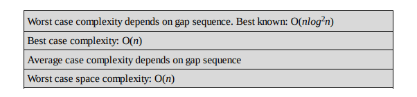
Performance
10.9 Merge Sort
Merge sort is an example of the divide and conquer strategy.
Important Notes
• Merging is the process of combining two sorted files to make one bigger sorted file.
• Selection is the process of dividing a file into two parts: k smallest elements and n – k largest elements.
• Selection and merging are opposite operations ○ selection splits a list into two lists ○ merging joins two files to make one file
• Merge sort is Quick sort’s complement
• Merge sort accesses the data in a sequential manner
• This algorithm is used for sorting a linked list
• Merge sort is insensitive to the initial order of its input
• In Quick sort most of the work is done before the recursive calls. Quick sort starts with the largest subfile and finishes with the small ones and as a result it needs stack. Moreover, this algorithm is not stable. Merge sort divides the list into two parts; then each part is conquered individually. Merge sort starts with the small subfiles and finishes with the largest one. As a result it doesn’t need stack. This algorithm is stable.
Implementation
}
void Mergesort(int a[], int temp[], int left, int right){
int mid; if(right > left) {
mid (right + left) / 2; Mergesort(A, temp, left, mid);
Mergesort(A, temp, mid+1, right);
Merge(A, temp, left, mid+1, right);
void Merge(int A[], int temp[], int left, int mid, int right) {
int i, left end, size, temp_pos;
left_end mid-1;
temp_pos = left;
size = right - left + 1;
while ((left <= left end) && (mid <= right)) {
if(A[left] <= Amid]) {
temp[temp_pos] =A[left];
temp_pos temp_pos + 1; left-left+1;
}
else{
temp[temp_pos] =A[mid];
temp_pos = temp_pos + 1;
mid = mid + 1;
while (left <= left_end) {
}
temp[temp_pos] A[left];
left left+1;
temp_pos temp_pos + 1;
while (mid <= right) {
}
temp[temp_pos] = A[mid];
mid = mid + 1;
temp_pos temp_pos + 1;
for (i=0; i < size; i++){
A[right] = temp[right];
right = right - 1;
Analysis
In Merge sort the input list is divided into two parts and these are solved recursively. After solving the sub problems, they are merged by scanning the resultant sub problems. Let us assume T(n) is the complexity of Merge sort with n elements. The recurrence for the Merge Sort can be defined as:
Recurrence for Mergesort is T(n) = 2T() + O(n). Using Master theorem, we get, T(n) = O(nlogn).
Note: For more details, refer to Divide and Conquer chapter.
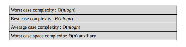
Performance
10.10 Heap Sort
Heapsort is a comparison-based sorting algorithm and is part of the selection sort family. Although somewhat slower in practice on most machines than a good implementation of Quick sort, it has the advantage of a more favorable worst-case Θ(nlogn) runtime. Heapsort is an inplace algorithm but is not a stable sort.
Performance
For other details on Heapsort refer to the Priority Queues chapter.
10.11 Quicksort
Quick sort is an example of a divide-and-conquer algorithmic technique. It is also called partition exchange sort. It uses recursive calls for sorting the elements, and it is one of the famous algorithms among comparison-based sorting algorithms.
Divide: The array A[low …high] is partitioned into two non-empty sub arrays A[low …q] and A[q + 1… high], such that each element of A[low … high] is less than or equal to each element of A[q + 1… high]. The index q is computed as part of this partitioning procedure.
Conquer: The two sub arrays A[low …q] and A[q + 1 …high] are sorted by recursive calls to Quick sort
Algorithm
The recursive algorithm consists of four steps:
1) If there are one or no elements in the array to be sorted, return.
2) Pick an element in the array to serve as the “pivot” point. (Usually the left-most element in the array is used.)
3) Split the array into two parts – one with elements larger than the pivot and the other with elements smaller than the pivot.
4) Recursively repeat the algorithm for both halves of the original array.
Implementation
void Counting Sort (int A[], int n, int B[], int K) { int C[K], i, j; //Complexity: O(K) for (i=0; i<K; i++) C[i] = 0;
//Complexity: O(n) for (j=0; j<n; j++)
C[AU]] = C[AG]] + 1;
//C[i] now contains the number of elements equal to i
//Complexity: O(K)
for (i=1; i<K; i++)
C[i] - Ci] + C[i-1];
// C[i] now contains the number of elements ≤ i //Complexity: O(n)
for (jn-1; j=0;j--) {
B[C[A]]] = AG]; C[AU]] = C[AU]] - 1;
}
Analysis
Let us assume that T(n) be the complexity of Quick sort and also assume that all elements are distinct. Recurrence for T(n) depends on two subproblem sizes which depend on partition element. If pivot is i th smallest element then exactly (i – 1) items will be in left part and (n – i) in right part. Let us call it as i –split. Since each element has equal probability of selecting it as pivot the probability of selecting i th element is n/2 .
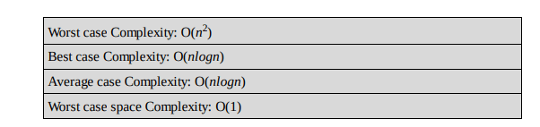
Best Case: Each partition splits array in halves and gives
T(n) = 2T(n/2) + Θ(n) = Θ(nlogn), [using Divide and Conquer master theorem]
Worst Case: Each partition gives unbalanced splits and we get
T(n) = T(n – 1) + Θ(n) = Θ(n 2 )[using Subtraction and Conquer master theorem]
The worst-case occurs when the list is already sorted and last element chosen as pivot.
Average Case: In the average case of Quick sort, we do not know where the split happens. For this reason, we take all possible values of split locations, add all their complexities and divide with n to get the average case complexity
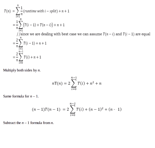
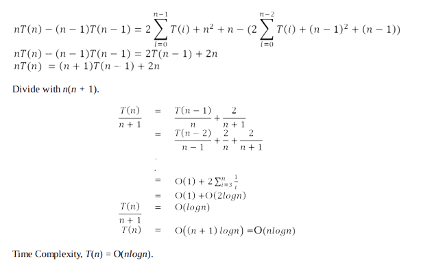
Performance
Randomized Quick sort
In average-case behavior of Quick sort, we assume that all permutations of the input numbers are equally likely. However, we cannot always expect it to hold. We can add randomization to an algorithm in order to reduce the probability of getting worst case in Quick sort.
There are two ways of adding randomization in Quick sort: either by randomly placing the input data in the array or by randomly choosing an element in the input data for pivot. The second choice is easier to analyze and implement. The change will only be done at the partition algorithm.
In normal Quick sort, pivot element was always the leftmost element in the list to be sorted. Instead of always using A[low] as pivot, we will use a randomly chosen element from the subarray A[low..high] in the randomized version of Quick sort. It is done by exchanging element A[low] with an element chosen at random from A[low..high]. This ensures that the pivot element is equally likely to be any of the high – low + 1 elements in the subarray.
Since the pivot element is randomly chosen, we can expect the split of the input array to be reasonably well balanced on average. This can help in preventing the worst-case behavior of quick sort which occurs in unbalanced partitioning. Even though the randomized version improves the worst case complexity, its worst case complexity is still O(n 2 ). One way to improve Randomized – Quick sort is to choose the pivot for partitioning more carefully than by picking a random element from the array. One common approach is to choose the pivot as the median of a set of 3 elements randomly selected from the array.
10.12 Tree Sort
Tree sort uses a binary search tree. It involves scanning each element of the input and placing it into its proper position in a binary search tree. This has two phases:
• First phase is creating a binary search tree using the given array elements.
• Second phase is traversing the given binary search tree in inorder, thus resulting in a sorted array.
Performance
The average number of comparisons for this method is O(nlogn). But in worst case, the number of comparisons is reduced by O(n 2 ), a case which arises when the sort tree is skew tree.
10.13 Comparison of Sorting Algorithms
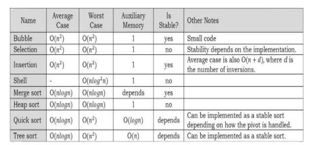
Note: n denotes the number of elements in the input.
10.14 Linear Sorting Algorithms
In earlier sections, we have seen many examples of comparison-based sorting algorithms. Among them, the best comparison-based sorting has the complexity O(nlogn). In this section, we will discuss other types of algorithms: Linear Sorting Algorithms. To improve the time complexity of sorting these algorithms, we make some assumptions about the input. A few examples of Linear Sorting Algorithms are:
• Counting Sort
• Bucket Sort
• Radix Sort
10.15 Counting Sort
Counting sort is not a comparison sort algorithm and gives O(n) complexity for sorting. To achieve O(n) complexity, counting sort assumes that each of the elements is an integer in the range 1 to K, for some integer K. When if = O(n), the counting sort runs in O(n) time. The basic idea of Counting sort is to determine, for each input element X, the number of elements less than X. This information can be used to place it directly into its correct position. For example, if 10 elements are less than X, then X belongs to position 11 in the output.
In the code below, A[0 ..n – 1] is the input array with length n. In Counting sort we need two more arrays: let us assume array B[0 ..n – 1] contains the sorted output and the array C[0 ..K – 1] provides temporary storage.
void Quicksort( int A[], int low, int high) { int pivot;
}
}
/* Termination condition! */
if( high >low) {
pivot = Partition( A, low, high ); Quicksort( A, low, pivot-1); Quicksort( A, pivot+1, high );
int Partition( int A, int low, int high) {
int left, right, pivot_item =A[low];
left = low;
right = high;
while (left < right){
}
/* Move left while item < pivot */ while( A[left] < pivot_item) left++;
/* Move right while item > pivot */ while( A[right]> pivot_item) right--;
if(left < right)
swap(A,left, right);
/* right is final position for the pivot */
A[low] =A[right];
A[right] = pivot_item;
return right;
Total Complexity: O(K) + O(n) + O(K) + O(n) = O(n) if K =O(n). Space Complexity: O(n) if K =O(n).
Note: Counting works well if K =O(n). Otherwise, the complexity will be greater.
10.16 Bucket Sort (or Bin Sort)
Like Counting sort, Bucket sort also imposes restrictions on the input to improve the performance. In other words, Bucket sort works well if the input is drawn from fixed set. Bucket sort is the generalization of Counting Sort. For example, assume that all the input elements from {0, 1, . . . , K – 1}, i.e., the set of integers in the interval [0, K – 1]. That means, K is the number of distant elements in the input. Bucket sort uses K counters. The i th counter keeps track of the number of occurrences of the i th element. Bucket sort with two buckets is effectively a version of Quick sort with two buckets.
For bucket sort, the hash function that is used to partition the elements need to be very good and must produce ordered hash: if i < k then hash(i) < hash(k). Second, the elements to be sorted must be uniformly distributed.
The aforementioned aside, bucket sort is actually very good considering that counting sort is reasonably speaking its upper bound. And counting sort is very fast. The particular distinction for bucket sort is that it uses a hash function to partition the keys of the input array, so that multiple keys may hash to the same bucket. Hence each bucket must effectively be a growable list; similar to radix sort.
In the below code insertionsort is used to sort each bucket. This is to inculcate that the bucket sort algorithm does not specify which sorting technique to use on the buckets. A programmer may choose to continuously use bucket sort on each bucket until the collection is sorted (in the manner of the radix sort program below). Whichever sorting method is used on the , bucket sort still tends toward O(n).
int Check DuplicatesInArray(in A[], int n) { for (int i = 0; i < n; i++) for (int j=i+1;j< n; j++) if(A[i]==A[i])
return false;
reutrn true;
Time Complexity: O(n). Space Complexity: O(n).
10.17 Radix Sort
Similar to Counting sort and Bucket sort, this sorting algorithm also assumes some kind of information about the input elements. Suppose that the input values to be sorted are from base d. That means all numbers are d-digit numbers.
In Radix sort, first sort the elements based on the last digit [the least significant digit]. These results are again sorted by second digit [the next to least significant digit]. Continue this process for all digits until we reach the most significant digits. Use some stable sort to sort them by last digit. Then stable sort them by the second least significant digit, then by the third, etc. If we use Counting sort as the stable sort, the total time is O(nd) ≈ O(n).
Algorithm:
1) Take the least significant digit of each element.
2) Sort the list of elements based on that digit, but keep the order of elements with the same digit (this is the definition of a stable sort).
3) Repeat the sort with each more significant digit.
The speed of Radix sort depends on the inner basic operations. If the operations are not efficient enough, Radix sort can be slower than other algorithms such as Quick sort and Merge sort. These operations include the insert and delete functions of the sub-lists and the process of isolating the digit we want. If the numbers are not of equal length then a test is needed to check for additional digits that need sorting. This can be one of the slowest parts of Radix sort and also one of the hardest to make efficient.
Since Radix sort depends on the digits or letters, it is less flexible than other sorts. For every different type of data, Radix sort needs to be rewritten, and if the sorting order changes, the sort needs to be rewritten again. In short, Radix sort takes more time to write, and it is very difficult to write a general purpose Radix sort that can handle all kinds of data.
For many programs that need a fast sort, Radix sort is a good choice. Still, there are faster sorts, which is one reason why Radix sort is not used as much as some other sorts.
Time Complexity: O(nd) ≈ O(n), if d is small.
10.18 Topological Sort
Refer to Graph Algorithms
Chapter. 10.19 External Sorting
External sorting is a generic term for a class of sorting algorithms that can handle massive amounts of data. These external sorting algorithms are useful when the files are too big and cannot fit into main memory.
As with internal sorting algorithms, there are a number of algorithms for external sorting. One such algorithm is External Mergesort. In practice, these external sorting algorithms are being supplemented by internal sorts.
Simple External Mergesort
A number of records from each tape are read into main memory, sorted using an internal sort, and then output to the tape. For the sake of clarity, let us assume that 900 megabytes of data needs to be sorted using only 100 megabytes of RAM.
1) Read 100MB of the data into main memory and sort by some conventional method (let us say Quick sort).
2) Write the sorted data to disk.
3) Repeat steps 1 and 2 until all of the data is sorted in chunks of 100MB. Now we need to merge them into one single sorted output file.
4) Read the first 10MB of each sorted chunk (call them input buffers) in main memory (90MB total) and allocate the remaining 10MB for output buffer.
5) Perform a 9-way Mergesort and store the result in the output buffer. If the output buffer is full, write it to the final sorted file. If any of the 9 input buffers gets empty, fill it with the next 10MB of its associated 100MB sorted chunk; or if there is no more data in the sorted chunk, mark it as exhausted and do not use it for merging.

The above algorithm can be generalized by assuming that the amount of data to be sorted exceeds the available memory by a factor of K. Then, K chunks of data need to be sorted and a K -way merge has to be completed.
If X is the amount of main memory available, there will be K input buffers and 1 output buffer of size X/(K + 1) each. Depending on various factors (how fast is the hard drive?) better performance can be achieved if the output buffer is made larger (for example, twice as large as one input buffer).
Complexity of the 2-way External Merge sort: In each pass we read + write each page in file. Let us assume that there are n pages in file. That means we need ⌈logn⌉ + 1 number of passes. The total cost is 2n(⌈logn⌉ + 1).
10.20 Sorting: Problems & Solutions
Problem-1 Given an array A[0…n– 1] of n numbers containing the repetition of some number. Give an algorithm for checking whether there are repeated elements or not. Assume that we are not allowed to use additional space (i.e., we can use a few temporary variables, O(1) storage).
Solution: Since we are not allowed to use extra space, one simple way is to scan the elements one-by-one and for each element check whether that element appears in the remaining elements. If we find a match we return true.
#define BUCKETS 10
void BucketSort(int A[], int array_size) { int i, j, k;
int buckets[BUCKETS]; for(j=0; j< BUCKETS; j++) buckets[j] = 0;
for(i=0; i< array_size; i++)
++ buckets[A[i]];
for(i =0,j=0; j< BUCKETS; j++) for(k = buckets[j];k> 0; --k) A[i++]=j;
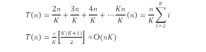
Each iteration of the inner, j-indexed loop uses O(1) space, and for a fixed value of i, the j loop executes n – i times. The outer loop executes n – 1 times, so the entire function uses time proportional to

Time Complexity: O(n 2 ). Space Complexity: O(1).
Problem-2 Can we improve the time complexity of Problem-1?
Solution: Yes, using sorting technique.
int Check DuplicatesInArray(in A[], int n) {
//for heap sort algorithm refer Priority Queues chapter Heapsort( A, n );
for (int i = 0; i < n-1; i++) if(A[i]==A[i+1])
reutrn true;
return false;
Heapsort function takes O(nlogn) time, and requires O(1) space. The scan clearly takes n – 1 iterations, each iteration using O(1) time. The overall time is O(nlogn + n) = O(nlogn).
Time Complexity: O(nlogn). Space Complexity: O(1).
Note: For variations of this problem, refer Searching chapter.
Problem-3 Given an array A[0 …n – 1], where each element of the array represents a vote in the election. Assume that each vote is given as an integer representing the ID of the chosen candidate. Give an algorithm for determining who wins the election.
Solution: This problem is nothing but finding the element which repeated the maximum number of times. The solution is similar to the Problem-1 solution: keep track of counter.
int Check WhoWins The Election(in A[], int n) { int i, j, counter = 0, maxCounter = 0, candidate; candidate = A[0];
for (i=0; i < n; i++){
candidate = A[i];
counter = 0;
for (j=i+1;j< n; j++) {
}
if(A[i]==A[j]) counter++;
if(counter > maxCounter) {
return candidate;
maxCounter counter;
candidate - A[i];
Time Complexity: O(n 2 ). Space Complexity: O(1).
Note: For variations of this problem, refer to Searching chapter.
Problem-4 Can we improve the time complexity of Problem-3? Assume we don’t have any extra space.
Solution: Yes. The approach is to sort the votes based on candidate ID, then scan the sorted array and count up which candidate so far has the most votes. We only have to remember the winner, so we don’t need a clever data structure. We can use Heapsort as it is an in-place sorting algorithm.
int Check WhoWins The Election (in A[], int n) { int i, j, currentCounter = 1, maxCounter = 1; int current Candidate, maxCandidate; currentCandidate maxCandidate= A[0];
//for heap sort algorithm refer Priority Queues Chapter Heapsort(A, n);
i
for (int i = 1; i < n; i++) {
if( A[i]== currentCandidate)
currentCounter++;
else{
currentCandidate = A[i];
currentCounter = 1;
}
if(currentCounter > maxCounter)
maxCounter = currentCounter;
else{
maxCandidate currentCandidate; maxCounter = currentCounter;
return candidate;
Since Heapsort time complexity is O(nlogn) and in-place, it only uses an additional O(1) of storage in addition to the input array. The scan of the sorted array does a constant-time conditional n – 1 times, thus using O(n) time. The overall time bound is O(nlogn).
Problem-5 Can we further improve the time complexity of Problem-3?
Solution: In the given problem, the number of candidates is less but the number of votes is significantly large. For this problem we can use counting sort.
Time Complexity: O(n), n is the number of votes (elements) in the array. Space Complexity: O(k), k is the number of candidates participating in the election.
Problem-6 Given an array A of n elements, each of which is an integer in the range [1, n 2 ], how do we sort the array in O(n) time?
Solution: If we subtract each number by 1 then we get the range [0, n 2 – 1]. If we consider all numbers as 2 –digit base n. Each digit ranges from 0 to n 2 – 1. Sort this using radix sort. This uses only two calls to counting sort. Finally, add 1 to all the numbers. Since there are 2 calls, the complexity is O(2n) ≈ O(n).
Problem-7 For Problem-6, what if the range is [1… n 3 ]?
Solution: If we subtract each number by 1 then we get the range [0, n 3 – 1]. Considering all numbers as 3-digit base n: each digit ranges from 0 to n 3 – 1. Sort this using radix sort. This uses only three calls to counting sort. Finally, add 1 to all the numbers. Since there are 3 calls, the complexity is O(3n) ≈ O(n).
Problem-8 Given an array with n integers, each of value less than n 100 , can it be sorted in linear time?
Solution: Yes. The reasoning is same as in of Problem-6 and Problem-7.
Problem-9 Let A and B be two arrays of n elements each. Given a number K, give an O(nlogn) time algorithm for determining whether there exists a ∈ A and b ∈ B such that a + b = K.
Solution: Since we need O(nlogn), it gives us a pointer that we need to sort. So, we will do that.
int Find( int A[], int B[], int n, K) {
int i, c; Heapsort( A, n);
// O(nlogn)
for (i=0; i< n; i++) {
// O(n)
c-k-Bli];
// 0(1)
if(BinarySearch(A, c)) return 1;
// O(logn)
}
return 0;
Note: For variations of this problem, refer to Searching chapter.
Problem-10 Let A,B and C be three arrays of n elements each. Given a number K, give an O(nlogn) time algorithm for determining whether there exists a ∈ A, b ∈ B and c ∈ C such that a + b + c = K.
Solution: Refer to Searching chapter.
Problem-11 Given an array of n elements, can we output in sorted order the K elements following the median in sorted order in time O(n + KlogK).
Solution: Yes. Find the median and partition the median. With this we can find all the elements greater than it. Now find the K th largest element in this set and partition it; and get all the elements less than it. Output the sorted list of the final set of elements. Clearly, this operation takes O(n + KlogK) time.
Problem-12 Consider the sorting algorithms: Bubble sort, Insertion sort, Selection sort, Merge sort, Heap sort, and Quick sort. Which of these are stable?
Solution: Let us assume that A is the array to be sorted. Also, let us say R and S have the same key and R appears earlier in the array than S. That means, R is at A[i] and S is at A[j], with i < j. To show any stable algorithm, in the sorted output R must precede S.
Bubble sort: Yes. Elements change order only when a smaller record follows a larger. Since S is not smaller than R it cannot precede it.
Selection sort: No. It divides the array into sorted and unsorted portions and iteratively finds the minimum values in the unsorted portion. After finding a minimum x, if the algorithm moves x into the sorted portion of the array by means of a swap, then the element swapped could be R which then could be moved behind S. This would invert the positions of R and S, so in general it is not stable. If swapping is avoided, it could be made stable but the cost in time would probably be very significant.
Insertion sort: Yes. As presented, when S is to be inserted into sorted subarray A[1..j – 1], only records larger than S are shifted. Thus R would not be shifted during S’s insertion and hence would always precede it.
Merge sort: Yes, In the case of records with equal keys, the record in the left subarray gets preference. Those are the records that came first in the unsorted array. As a result, they will precede later records with the same key.
Heap sort: No. Suppose i = 1 and R and S happen to be the two records with the largest keys in the input. Then R will remain in location 1 after the array is heapified, and will be placed in location n in the first iteration of Heapsort. Thus S will precede R in the output.
Quick sort: No. The partitioning step can swap the location of records many times, and thus two records with equal keys could swap position in the final output.
Problem-13 Consider the same sorting algorithms as that of Problem-12. Which of them are in-place?
Solution: Bubble sort: Yes, because only two integers are required. Insertion sort: Yes, since we need to store two integers and a record.
Selection sort: Yes. This algorithm would likely need space for two integers and one record.
Merge sort: No. Arrays need to perform the merge. (If the data is in the form of a linked list, the sorting can be done in-place, but this is a nontrivial modification.)
Heap sort: Yes, since the heap and partially-sorted array occupy opposite ends of the input array.
Quicksort: No, since it is recursive and stores O(logn) activation records on the stack. Modifying it to be non-recursive is feasible but nontrivial.
Problem-14 Among Quick sort, Insertion sort, Selection sort, and Heap sort algorithms, which one needs the minimum number of swaps?
Solution: Selection sort – it needs n swaps only (refer to theory section).
Problem-15 What is the minimum number of comparisons required to determine if an integer appears more than n/2 times in a sorted array of n integers?
Solution: Refer to Searching chapter.
Problem-16 Sort an array of 0’s, 1’s and 2’s: Given an array A[] consisting of 0’s, 1’s and 2’s, give an algorithm for sorting A[]. The algorithm should put all 0’s first, then all 1’s and all 2’s last. Example: Input = {0,1,1,0,1,2,1,2,0,0,0,1}, Output = {0,0,0,0,0,1,1,1,1,1,2,2}
Solution: Use Counting sort. Since there are only three elements and the maximum value is 2, we need a temporary array with 3 elements.
Time Complexity: O(n). Space Complexity: O(1).
Note: For variations of this problem, refer to Searching chapter.
Problem-17 Is there any other way of solving Problem-16?
Solution: Using Quick dort. Since we know that there are only 3 elements, 0,1 and 2 in the array, we can select 1 as a pivot element for Quick sort. Quick sort finds the correct place for 1 by moving all 0’s to the left of 1 and all 2’s to the right of 1. For doing this it uses only one scan.
Time Complexity: O(n). Space Complexity: O(1).
Note: For efficient algorithm, refer to Searching chapter.
Problem-18 How do we find the number that appeared the maximum number of times in an array?
Solution: One simple approach is to sort the given array and scan the sorted array. While scanning, keep track of the elements that occur the maximum number of times. Algorithm
QuickSort(A, n);
int i, j, count=1, Number=A[0], j=0; for(i=0;i<n;i++) {
if(Alj]==A){
count++;
Number=A[j];
}
j=i;
}
printf("Number:%d, count:%d", Number, count);
Time Complexity = Time for Sorting + Time for Scan = O(nlogn) +O(n) = O(nlogn). Space Complexity: O(1).
Note: For variations of this problem, refer to Searching chapter.
Problem-19 Is there any other way of solving Problem-18?
Solution: Using Binary Tree. Create a binary tree with an extra field count which indicates the number of times an element appeared in the input. Let us say we have created a Binary Search Tree [BST]. Now, do the In-Order traversal of the tree. The In-Order traversal of BST produces the sorted list. While doing the In-Order traversal keep track of the maximum element.
Time Complexity: O(n) + O(n) ≈ O(n). The first parameter is for constructing the BST and the second parameter is for Inorder Traversal. Space Complexity: O(2n) ≈ O(n), since every node in BST needs two extra pointers.
Problem-20 Is there yet another way of solving Problem-18?
Solution: Using Hash Table. For each element of the given array we use a counter, and for each occurrence of the element we increment the corresponding counter. At the end we can just return the element which has the maximum counter.
Time Complexity: O(n). Space Complexity: O(n). For constructing the hash table we need O(n).
Note: For the efficient algorithm, refer to the Searching chapter. Problem-21 Given a 2 GB file with one string per line, which sorting algorithm would we use to sort the file and why? Solution: When we have a size limit of 2GB, it means that we cannot bring all the data into the main memory.
Algorithm: How much memory do we have available? Let’s assume we have X MB of memory available. Divide the file into K chunks, where X * K ~ 2 GB.
• Bring each chunk into memory and sort the lines as usual (any O(nlogn) algorithm).
• Save the lines back to the file.
• Now bring the next chunk into memory and sort.
• Once we’re done, merge them one by one; in the case of one set finishing, bring more data from the particular chunk.
The above algorithm is also known as external sort. Step 3 – 4 is known as K-way merge. The idea behind going for an external sort is the size of data. Since the data is huge and we can’t bring it to the memory, we need to go for a disk-based sorting algorithm.
Problem-22 Nearly sorted: Given an array of n elements, each which is at most K positions from its target position, devise an algorithm that sorts in O(n logK) time.
Solution: Divide the elements into n/K groups of size K, and sort each piece in O(KlogK) time, let’s say using Mergesort. This preserves the property that no element is more than K elements out of position. Now, merge each block of K elements with the block to its left.
Problem-23 Is there any other way of solving Problem-22?
Solution: Insert the first K elements into a binary heap. Insert the next element from the array into the heap, and delete the minimum element from the heap. Repeat.
Problem-24 Merging K sorted lists: Given K sorted lists with a total of n elements, give an O(nlogK) algorithm to produce a sorted list of all n elements.
Solution: Simple Algorithm for merging K sorted lists: Consider groups each having n/k elements. Take the first list and merge it with the second list using a linear-time algorithm for merging two sorted lists, such as the merging algorithm used in merge sort. Then, merge the resulting list of 2n/k elements with the third list, and then merge the resulting list of 3n/k elements with the fourth list. Repeat this until we end up with a single sorted list of all n elements.
Time Complexity: In each iteration we are merging K elements.
Problem-25 Can we improve the time complexity of Problem-24?
Solution: One method is to repeatedly pair up the lists and then merge each pair. This method can also be seen as a tail component of the execution merge sort, where the analysis is clear. This is called the Tournament Method. The maximum depth of the Tournament Method is logK and in each iteration we are scanning all the n elements.
Time Complexity; O(nlogK).
Problem-26 Is there any other way of solving Problem-24?
Solution: The other method is to use a rain priority queue for the minimum elements of each of the if lists. At each step, we output the extracted minimum of the priority queue, determine from which of the K lists it came, and insert the next element from that list into the priority queue. Since we are using priority queue, that maximum depth of priority queue is logK.
Time Complexity; O(nlogK).
Problem-27 Which sorting method is better for Linked Lists?
Solution: Merge Sort is a better choice. At first appearance, merge sort may not be a good selection since the middle node is required to subdivide the given list into two sub-lists of equal length. We can easily solve this problem by moving the nodes alternatively to two lists (refer to Linked Lists chapter). Then, sorting these two lists recursively and merging the results into a single list will sort the given one.
typedef struct ListNode{ int data;
};
struct ListNode *next;
void Qsort(struct ListNode *first, struct ListNode * last) {
struct ListNode *lesHEAD=NULL, lesTAIL=NULL; struct ListNode *equHEAD=NULL, equTAIL-NULL; struct ListNode *larHEAD=NULL, larTAIL=NULL;
struct ListNode *current = *first;
int pivot, info;
if(current NULL) return;
pivot = current-data;
Append(current, equHEAD, equTAIL);
while (current != NULL) {
}
info = current-data;
if(info< pivot)
Append(current, lesHEAD, lesTAIL)
else if(info > pivot)
Append(current, larHEAD, larTAIL)
else Append(current, equHEAD, equTAIL);
Quicksort(&lesHEAD, &lesTAIL);
Quicksort(&larHEAD, &larTAIL);
Join(lesHEAD, lesTAIL,equHEAD, equTAIL); Join(lesHEAD, equTAIL,larHEAD, larTAIL); *first = lesHEAD;
*last = larTAIL;
Note: Append() appends the first argument to the tail of a singly linked list whose head and tail are defined by the second and third arguments.
All external sorting algorithms can be used for sorting linked lists since each involved file can be considered as a linked list that can only be accessed sequentially. We can sort a doubly linked list using its next fields as if it was a singly linked one and reconstruct the prev fields after sorting with an additional scan.
Problem-28 Can we implement Linked Lists Sorting with Quick Sort?
Solution: The original Quick Sort cannot be used for sorting Singly Linked Lists. This is because we cannot move backward in Singly Linked Lists. But we can modify the original Quick Sort and make it work for Singly Linked Lists.
Let us consider the following modified Quick Sort implementation. The first node of the input list is considered a pivot and is moved to equal. The value of each node is compared with the pivot and moved to less (respectively, equal or larger) if the nodes value is smaller than (respectively, equal to or larger than) the pivot. Then, less and larger are sorted recursively. Finally, joining less, equal and larger into a single list yields a sorted one.
Append() appends the first argument to the tail of a singly linked list whose head and tail are defined by the second and third arguments. On return, the first argument will be modified so that it points to the next node of the list. Join() appends the list whose head and tail are defined by the third and fourth arguments to the list whose head and tail are defined by the first and second arguments. For simplicity, the first and fourth arguments become the head and tail of the resulting list.
typedef struct ListNode{ int data;
};
struct ListNode *next;
struct ListNodeLinkedListMergeSort(struct ListNode * first) {
struct ListNode list 1 HEAD = NULL; struct ListNode list 1TAIL = NULL;
struct ListNode list 2HEAD = NULL; struct ListNode list2TAIL = NULL; if(first NULL || first-next--NULL) return first;
while (first != NULL) {
Append(first, list1 HEAD, list1TAIL); if(first!= NULL)
Append(first, list2HEAD, list2TAIL);
list 1 HEAD = LinkedListMergeSort(list1HEAD); list2HEAD = LinkedListMergeSort(list2HEAD); return Merge(list1 HEAD, list2HEAD);
Problem-29 Given an array of 100,000 pixel color values, each of which is an integer in the range [0,255]. Which sorting algorithm is preferable for sorting them?
Solution: Counting Sort. There are only 256 key values, so the auxiliary array would only be of size 256, and there would be only two passes through the data, which would be very efficient in both time and space.
Problem-30 Similar to Problem-29, if we have a telephone directory with 10 million entries, which sorting algorithm is best?
Solution: Bucket Sort. In Bucket Sort the buckets are defined by the last 7 digits. This requires an auxiliary array of size 10 million and has the advantage of requiring only one pass through the data on disk. Each bucket contains all telephone numbers with the same last 7 digits but with different area codes. The buckets can then be sorted by area code with selection or insertion sort; there are only a handful of area codes.
Problem-31 Give an algorithm for merging K-sorted lists.
Solution: Refer to Priority Queues chapter. Problem-32 Given a big file containing billions of numbers. Find maximum 10 numbers from this file. Solution: Refer to Priority Queues chapter.
Problem-33 There are two sorted arrays A and B. The first one is of size m + n containing only m elements. Another one is of size n and contains n elements. Merge these two arrays into the first array of size m + n such that the output is sorted.
Solution: The trick for this problem is to start filling the destination array from the back with the largest elements. We will end up with a merged and sorted destination array.
void Merge(int[] A[], int m, int B[], int n) { int count = m;
int i=n-1,j= count - 1, k = m -1; for(;k>=0;k--) {
if(B[i]> Aj] || j < 0) {
}
A[k] -B[i];
i--;
if(i<0)
break;
else {
A[k] = Alji];
j--;
Time Complexity: O(m + n). Space Complexity: O(1).
Problem-34 Nuts and Bolts Problem: Given a set of n nuts of different sizes and n bolts such that there is a one-to-one correspondence between the nuts and the bolts, find for each nut its corresponding bolt. Assume that we can only compare nuts to bolts: we cannot compare nuts to nuts and bolts to bolts.
Alternative way of framing the question: We are given a box which contains bolts and nuts. Assume there are n nuts and n bolts and that each nut matches exactly one bolt (and vice versa). By trying to match a bolt and a nut we can see which one is bigger, but we cannot compare two bolts or two nuts directly. Design an efficient algorithm for matching the nuts and bolts.
Solution: Brute Force Approach: Start with the first bolt and compare it with each nut until we find a match. In the worst case, we require n comparisons. Repeat this for successive bolts on all remaining gives O(n 2 ) complexity.
Problem-35 For Problem-34, can we improve the complexity?
Solution: In Problem-34, we got O(n 2 ) complexity in the worst case (if bolts are in ascending order and nuts are in descending order). Its analysis is the same as that of Quick Sort. The improvement is also along the same lines. To reduce the worst case complexity, instead of selecting the first bolt every time, we can select a random bolt and match it with nuts. This randomized selection reduces the probability of getting the worst case, but still the worst case is O(n 2 ).
Problem-36 For Problem-34, can we further improve the complexity?
Solution: We can use a divide-and-conquer technique for solving this problem and the solution is very similar to randomized Quick Sort. For simplicity let us assume that bolts and nuts are represented in two arrays B and N.
The algorithm first performs a partition operation as follows: pick a random boltB[t]. Using this bolt, rearrange the array of nuts into three groups of elements:
• First the nuts smaller than B[i]
• Then the nut that matches B[i], and
• Finally, the nuts larger than B[i].
Next, using the nut that matches B[i], perform a similar partition on the array of bolts. This pair of partitioning operations can easily be implemented in O(n) time, and it leaves the bolts and nuts nicely partitioned so that the “pivot” bolt and nut are aligned with each other and all other bolts and nuts are on the correct side of these pivots – smaller nuts and bolts precede the pivots, and larger nuts and bolts follow the pivots. Our algorithm then completes by recursively applying itself to the subarray to the left and right of the pivot position to match these remaining bolts and nuts. We can assume by induction on n that these recursive calls will properly match the remaining bolts.
To analyze the running time of our algorithm, we can use the same analysis as that of randomized Quick Sort. Therefore, applying the analysis from Quick Sort, the time complexity of our algorithm is O(nlogn). Alternative Analysis: We can solve this problem by making a small change to Quick Sort. Let us assume that we pick the last element as the pivot, say it is a nut. Compare the nut with only bolts as we walk down the array. This will partition the array for the bolts. Every bolt less than the partition nut will be on the left. And every bolt greater than the partition nut will be on the right.
While traversing down the list, find the matching bolt for the partition nut. Now we do the partition again using the matching bolt. As a result, all the nuts less than the matching bolt will be on the left side and all the nuts greater than the matching bolt will be on the right side. Recursively call on the left and right arrays.
The time complexity is O(2nlogn) ≈ O(nlogn).
Problem-37 Given a binary tree, can we print its elements in sorted order in O(n) time by performing an In-order tree traversal?
Solution: Yes, if the tree is a Binary Search Tree [BST]. For more details refer to Trees chapter.
Problem-38 Given an array of elements, convert it into an array such that A < B > C < D > E < F and so on.
Solution: Sort the array, then swap every adjacent element to get the final result.
convertArraytoSaw Tooth Wave(){
int Al]=(0,-6,9,13,10,-1,8,12,54,14,-5); int n = sizeof(A)/sizeof(A[0]), i = 1, temp; sort(A, A+n);
for(i=1; i < n; i+=2){
}
if (i>0&& A[i-1]> A[i]){
temp =A[i]; A[i]=A[i-1]; A[i-1] = temp;
if (i<n-1 && A[i] < A[i+1]){
temp = A[i]; A[i]=A[i+1]; A[i+1] = temp;
}
}
for(i=0; i < n; i++){
cout<<A[i]<< " ";
The time complexity is O(nlogn+n) ≈ O(nlogn), for sorting and a scan.
Problem-39 Can we do Problem-38 with O(n) time?
Solution: Make sure all even positioned elements are greater than their adjacent odd elements, and we don’t need to worry about odd positioned elements. Traverse all even positioned elements of input array, and do the following:
• If the current element is smaller than the previous odd element, swap previous and current.
• If the current element is smaller than the next odd element, swap next and current.
#include<algorithm> convertArraytoSaw Tooth Wave(){
int All (0,-6,9,13,10,-1,8,12,54,14,-5); int n= sizeof(A)/sizeof(A[0]), i = 1, temp; sort(A, A+n);
for(i=1; i < n; i+=2){
if(i+1 <n){
temp = A[i]; A[i]=A[i+1]; A[i+1] = temp;
}
}
for(i=0; i < n; i++){
printf("%d", A[i]);
}
The time complexity is O(n).
Problem-40 Merge sort uses
(a) Divide and conquer strategy
(b) Backtracking approach
(c) Heuristic search
(d) Greedy approach
Solution:
(a). Refer theory section.
Problem-41 Which of the following algorithm design techniques is used in the quicksort algorithm?
(a) Dynamic programming
(b) Backtracking
(c) Divide and conquer
(d) Greedy method
Solution:
(c). Refer theory section.
Problem-42 For merging two sorted lists of sizes m and n into a sorted list of size m+n, we required comparisons of
(a) O(m)
(b) O(n)
(c) O(m + n)
(d) O(logm + logn)
Solution:
(c). We can use merge sort logic. Refer theory section.
Problem-43 Quick-sort is run on two inputs shown below to sort in ascending order
(i) 1,2,3 ….n
(ii) n, n- 1, n-2, …. 2, 1
Let C1 and C2 be the number of comparisons made for the inputs (i) and (ii) respectively. Then,
(a) C1 < C2
(b) C1 > C2
(c) C1 = C2
(d) we cannot say anything for arbitrary n.
Solution:
(b). Since the given problems needs the output in ascending order, Quicksort on already sorted order gives the worst case (O(n 2 )). So, (i) generates worst case and (ii) needs fewer comparisons.
Problem-44 Give the correct matching for the following pairs:
(A) O(logn)
(B) O(n)
C) O(nlogn)
(D) O(n 2 ) (P) Selection (Q) Insertion sort (R) Binary search (S) Merge sort (a) A – R B – P C – Q – D – S (b) A – R B – P C – S D – Q (c) A – P B – R C – S D – Q (d) A – P B – S C – R D – Q
Solution:
(b). Refer theory section.
Problem-45 Let s be a sorted array of n integers. Let t(n) denote the time taken for the most efficient algorithm to determine if there are two elements with sum less than 1000 in s. which of the following statements is true?
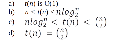
Solution:
(a). Since the given array is already sorted it is enough if we check the first two elements of the array.
Problem-46 The usual Θ(n 2 ) implementation of Insertion Sort to sort an array uses linear search to identify the position where an element is to be inserted into the already sorted part of the array. If, instead, we use binary search to identify the position, the worst case running time will
(a) remain Θ(n 2 )
(b) become Θ(n(log n) 2 )
(c) become Θ(nlogn)
(d) become Θ(n)
Solution:
(a). If we use binary search then there will be comparisons in the worst case, which is Θ(nlogn). But the algorithm as a whole will still have a running time of Θ(n 2 ) on average because of the series of swaps required for each insertion.
Problem-47 In quick sort, for sorting n elements, the n/4 th smallest element is selected as pivot using an O(n) time algorithm. What is the worst case time complexity of the quick sort?
(A) Θ(n)
(B) Θ(nLogn)
(C) Θ(n 2 )
(D) Θ(n 2 logn)
solution: The recursion expression becomes: T(n) = T(n/4) + T(3n/4) + en. Solving the recursion using variant of master theorem, we get Θ(nLogn).
Problem-48 Consider the Quicksort algorithm. Suppose there is a procedure for finding a pivot element which splits the list into two sub-lists each of which contains at least onefifth of the elements. Let T(n) be the number of comparisons required to sort n elements. Then
A) T (n) ≤ 2T (n /5) + n
B) T (n) ≤ T (n /5) + T (4n /5) + n
C) T (n) ≤ 2T (4n /5) + n
D) T (n) ≤ 2T (n /2) + n
Solution (C). For the case where n/5 elements are in one subset, T(n/5) comparisons are needed for the first subset with n/5 elements, T(4n/5) is for the rest 4n/5 elements, and n is for finding the pivot. If there are more than n/5 elements in one set then other set will have less than 4n/5 elements and time complexity will be less than T(n/5) + T(4n/5) + n.
Problem-49 Which of the following sorting algorithms has the lowest worst-case complexity?
(A) Merge sort
(B) Bubble sort
(C) Quick sort
(D) Selection sort
Solution: (A). Refer theory section.
Problem-50 Which one of the following in place sorting algorithms needs the minimum number of swaps?
(A) Quick sort
(B) Insertion sort
(C) Selection sort
(D) Heap sort
Solution: (C). Refer theory section.
Problem-51 You have an array of n elements. Suppose you implement quicksort by always choosing the central element of the array as the pivot. Then the tightest upper bound for the worst case performance is
(A) O(n 2 )
(B) O(nlogn)
(C) Θ(nlogn)
(D) O(n 3 )
Solution: (A). When we choose the first element as the pivot, the worst case of quick sort comes if the input is sorted- either in ascending or descending order.
Problem-52 Let P be a Quicksort Program to sort numbers in ascending order using the first element as pivot. Let t1 and t2 be the number of comparisons made by P for the inputs {1, 2, 3, 4, 5} and {4, 1, 5, 3, 2} respectively. Which one of the following holds?
(A) t1 = 5
(B) t1 < t2
(C) t1 > t2
(D) t1 = t2
Solution: (C). Quick Sort’s worst case occurs when first (or last) element is chosen as pivot with sorted arrays.
Problem-53 The minimum number of comparisons required to find the minimum and the maximum of 100 numbers is ——
Solution: 147 (Formula for the minimum number of comparisons required is 3n/2 – 3 with n numbers).
Problem-54 The number of elements that can be sorted in T(logn) time using heap sort is
(A) Θ(1)
(B) Θ(sqrt(logn))
(C) Θ(log n/(log log n))
(D) Θ(logn)
Solution: (D). Sorting an array with k elements takes time Θ(k log k) as k grows. We want to choose k such that Θ(k log k) = Θ(logn). Choosing k = Θ(logn) doesn’t necessarily work, since Θ(k log k) = Θ(logn loglogn) ≠ Θ(logn). On the other hand, if you choose k = T(log n / log log n), then the runtime of the sort will be
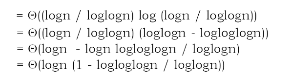
Notice that 1 – logloglogn / loglogn tends toward 1 as n goes to infinity, so the above expression actually is Θ(log n), as required. Therefore, if you try to sort an array of size Θ(logn / loglogn) using heap sort, as a function of n, the runtime is Θ(logn).
Problem-55 Which one of the following is the tightest upper bound that represents the number of swaps required to sort n numbers using selection sort?
(A) O(logn)
(B) O(n)
(C) O(nlogn)
(D) O(n 2 )
Solution: (B). Selection sort requires only O(n) swaps.
Problem-56 Which one of the following is the recurrence equation for the worst case time complexity of the Quicksort algorithm for sorting n(≥ 2) numbers? In the recurrence equations given in the options below, c is a constant.
(A)T(n) = 2T (n/2) + cn
(B) T(n) = T(n – 1) + T(0) + cn
(C) T(n) = 2T (n – 2) + cn
(D) T(n) = T(n/2) + cn
Solution: (B). When the pivot is the smallest (or largest) element at partitioning on a block of size n the result yields one empty sub-block, one element (pivot) in the correct place and sub block of size n – 1.
Problem-57 True or False. In randomized quicksort, each key is involved in the same number of comparisons.
Solution: False.
Problem-58 True or False: If Quicksort is written so that the partition algorithm always uses the median value of the segment as the pivot, then the worst-case performance is O(nlogn).
Soution: True.