8.1 Introduction In this chapter, we will represent an important mathematics concept: sets. This means how to represent a group of elements which do not need any order. The disjoint sets ADT is the one used for this purpose. It is used for solving the equivalence problem. It is very simple to implement. A simple array can be used for the implementation and each function takes only a few lines of code. Disjoint sets ADT acts as an auxiliary data structure for many other algorithms (for example, Kruskal’s algorithm in graph theory). Before starting our discussion on disjoint sets ADT, let us look at some basic properties of sets.
8.2 Equivalence Relations and Equivalence Classes
For the discussion below let us assume that 5 is a set containing the elements and a relation R is defined on it. That means for every pair of elements in a,b ∈ 5, a R b is either true or false. If a R b is true, then we say a is related to b, otherwise a is not related to b. A relation R is called an equivalence relation if it satisfies the following properties:
• Reflexive: For every element a ∈ S.aR a is true.
• Symmetric: For any two elements a, b ∈ S, if a R b is true then b R a is true.
• Transitive: For any three elements a, b, c ∈ S, if a R b and b R c are true then a R c is true.
As an example, relations ≤ (less than or equal to) and ≥ (greater than or equal to) on a set of integers are not equivalence relations. They are reflexive (since a ≤ a) and transitive (a ≤ b and b ≤ c implies a ≤ c) but not symmetric (a ≤ b does not imply b ≤ a).
Similarly, rail connectivity is an equivalence relation. This relation is reflexive because any location is connected to itself. If there is connectivity from city a to city b, then city b also has connectivity to city a, so the relation is symmetric. Finally, if city a is connected to city b and city b is connected to city c, then city a is also connected to city c
The equivalence class of an element a ∈ S is a subset of S that contains all the elements that are related to a. Equivalence classes create a partition of S. Every member of S appears in exactly one equivalence class. To decide if a R b, we just need to check whether a and b are in the same equivalence class (group) or not.
In the above example, two cities will be in same equivalence class if they have rail connectivity. If they do not have connectivity then they will be part of different equivalence classes
Since the intersection of any two equivalence classes is empty (ϕ), the equivalence classes are sometimes called disjoint sets. In the subsequent sections, we will try to see the operations that can be performed on equivalence classes. The possible operations are:
• Creating an equivalence class (making a set)
• Finding the equivalence class name (Find)
• Combining the equivalence classes (Union)
8.3 Disjoint Sets ADT To manipulate
the set elements we need basic operations defined on sets. In this chapter, we concentrate on the following set operations:
• MAKESET(X): Creates a new set containing a single element X.
• UNION(X, Y): Creates a new set containing the elements X and Y in their union and deletes the sets containing the elements X and Y.
• FIND(X): Returns the name of the set containing the element X.
8.4 Applications Disjoint sets
ADT have many applications and a few of them are:
• To represent network connectivity
• Image processing
• To find least common ancestor
• To define equivalence of finite state automata
• Kruskal’s minimum spanning tree algorithm (graph theory)
• In game algorithms
8.5 Tradeoffs in Implementing Disjoint Sets ADT
Let us see the possibilities for implementing disjoint set operations. Initially, assume the input elements are a collection of n sets, each with one element. That means, initial representation assumes all relations (except reflexive relations) are false. Each set has a different element, so that Si ∩ Sj= ф. This makes the sets disjoint.
To add the relation a R b (UNION), we first need to check whether a and b are already related or not. This can be verified by performing FINDs on both a and b and checking whether they are in the same equivalence class (set) or not.
If they are not, then we apply UNION. This operation merges the two equivalence classes containing a and b into a new equivalence class by creating a new set Sk = Si ∪ Sj and deletes Si and Sj . Basically there are two ways to implement the above FIND/UNION operations:
• Fast FIND implementation (also called Quick FIND)
• Fast UNION operation implementation (also called Quick UNION)
8.6 Fast FIND Implementation (Quick FIND)
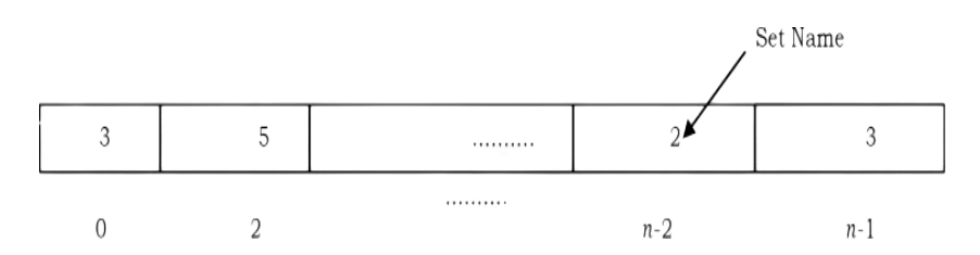
In this method, we use an array. As an example, in the representation below the array contains the set name for each element. For simplicity, let us assume that all the elements are numbered sequentially from 0 to n – 1.
In the example below, element 0 has the set name 3, element 1 has the set name 5, and so on. With this representation FIND takes only O(1) since for any element we can find the set name by accessing its array location in constant time.
In this representation, to perform UNION(a, b) [assuming that a is in set i and b is in set j] we need to scan the complete array and change all i’s to j. This takes O(n).
A sequence of n – 1 unions take O(n 2 ) time in the worst case. If there are O(n 2 ) FIND operations, this performance is fine, as the average time complexity is O(1) for each UNION or FIND operation. If there are fewer FINDs, this complexity is not acceptable.
8.7 Fast UNION Implementation (Quick UNION)
In this and subsequent sections, we will discuss the faster UNION implementations and its variants. There are different ways of implementing this approach and the following is a list of a few of them.
• Fast UNION implementations (Slow FIND)
• Fast UNION implementations (Quick FIND)
• Fast UNION implementations with path compression
8.8 Fast UNION Implementation (Slow FIND)
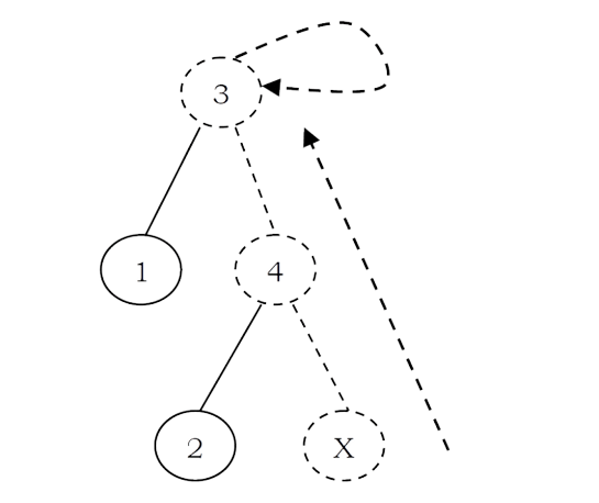
As we have discussed, FIND operation returns the same answer (set name) if and only if they are in the same set. In representing disjoint sets, our main objective is to give a different set name for each group. In general we do not care about the name of the set. One possibility for implementing the set is tree as each element has only one root and we can use it as the set name.
How are these represented? One possibility is using an array: for each element keep the root as its set name. But with this representation, we will have the same problem as that of FIND array implementation. To solve this problem, instead of storing the root we can keep the parent of the element. Therefore, using an array which stores the parent of each element solves our problem.
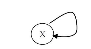
To differentiate the root node, let us assume its parent is the same as that of the element in the array. Based on this representation, MAKESET, FIND, UNION operations can be defined as:
• (X): Creates a new set containing a single element X and in the array update the parent of X as X. That means root (set name) of X is X.
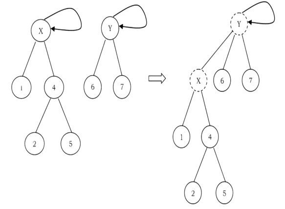
• UNION(X, Y): Replaces the two sets containing X and Y by their union and in the array updates the parent of X as Y.
• FIND(X): Returns the name of the set containing the element X. We keep on searching for X’s set name until we come to the root of the tree.
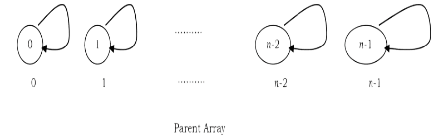
For the elements 0 to n – 1 the initial representation is:
To perform a UNION on two sets, we merge the two trees by making the root of one tree point to the root of the other.
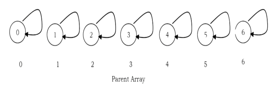
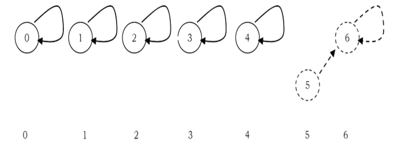
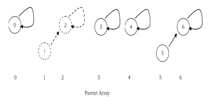
Initial Configuration for the elements 0 to 6
after UNION (5.6)
after U NION (1,2)
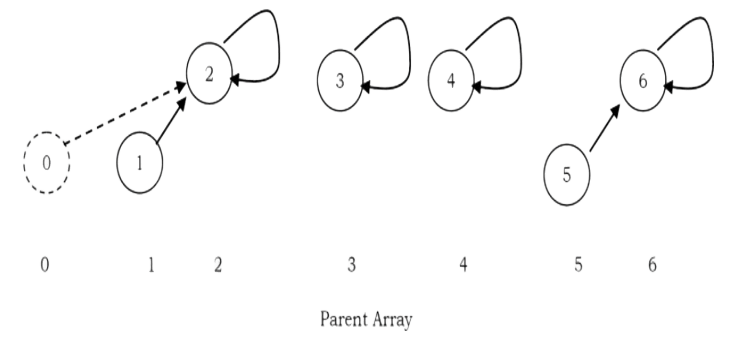
after UNION (0.2)
int FIND(int S[], int size, int X) { if(!(X >= 0 && X < size)) return -1; if( S[X] == X)
return X;
else return FIND(S, S[X]);
One important thing to observe here is, UNION operation is changing the root’s parent only, but not for all the elements in the sets. Due to this, the time complexity of UNION operation is O(1).
A FIND(X) on element X is performed by returning the root of the tree containing X. The time to perform this operation is proportional to the depth of the node representing X
Using this method, it is possible to create a tree of depth n – 1 (Skew Trees). The worst-case running time of a FIND is O(n) and m consecutive FIND operations take O(mn) time in the worst case.
MAKESET
void UNION( int S[], int size, int root], int root2){ if(FIND(S, size, root1)== FIND(S, size, root2)) return;
if(!((root] >= 0 && root1 < size) && (root2 >= 0 && root2 < size)))
return; S[root]]-root2;
FIND
void MAKESET( int S[], int size) { for(int i= size-1; i >=0; i--) S[i] = i;
UNION
void MAKESET( int S[], int size) { for(int i= size-1; i >= 0; i--) S[i] = -1;
8.9 Fast UNION Implementations (Quick FIND)
The main problem with the previous approach is that, in the worst case we are getting the skew trees and as a result the FIND operation is taking O(n) time complexity. There are two ways to improve it:
• UNION by Size (also called UNION by Weight): Make the smaller tree a subtree ofN the larger tree
• UNION by Height (also called UNION by Rank): Make the tree with less height a subtree of the tree with more height
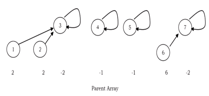
UNION by Size
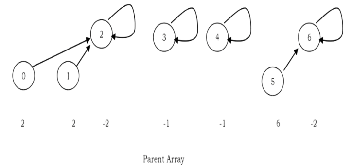
In the earlier representation, for each element i we have stored i (in the parent array) for the root element and for other elements we have stored the parent of i. But in this approach we store negative of the size of the tree (that means, if the size of the tree is 3 then store –3 in the parent array for the root element). For the previous example (after UNION(0,2)), the new representation will look like:

Assume that the size of one element set is 1 and store – 1. Other than this there is no change.
MAKESET
int FIND(int S[], int size, int X) { if(!(X >= 0 && X < size))) return -1;
if( S[X] == -1) return X;
else return FIND(S, S[X]);
FIND
void UNION( int S[], int size, int root1, int root2){ if(FIND(S, size, root1)== FIND(S, size, root2)) return;
if(!(root] >= 0 && root1 < size) && (root2 >= 0 && root2 < size)))
return; S[root1]=root2;
UNION by Size
int FIND(int S[], int size, int X) { if(!(X >= 0 && X < size)) return; if( S[X] <= 0) return X;
else return(S[X] = FIND(S, S[X]));
Note: There is no change in FIND operation implementation.
UNION by Height (UNION by Rank)
UNION by Height
void UNIONBySize(int S[], int size, int root], int root2){
if((FIND(S, size, root1) == FIND(S, size, root2)) && FIND(S, size, root1) != -1)
return;
if( S[root2] < S[root]) { S[root]] = root2;
S[root2] += S[root];
}
else{
S[root2]=root];
S[root1] += S[root2];
Note: For FIND operation there is no change in the implementation.
Comparing UNION by Size and UNION by Height
With UNION by size, the depth of any node is never more than logn. This is because a node is initially at depth 0. When its depth increases as a result of a UNION, it is placed in a tree that is at least twice as large as before. That means its depth can be increased at most logn times. This means that the running time for a FIND operation is O(logn), and a sequence of m operations takes O(m logn).
Similarly with UNION by height, if we take the UNION of two trees of the same height, the height of the UNION is one larger than the common height, and otherwise equal to the max of the two heights. This will keep the height of tree of n nodes from growing past O(logn). A sequence of m UNIONs and FINDs can then still cost O(m logn).
Path Compression
FIND operation traverses a list of nodes on the way to the root. We can make later FIND operations efficient by making each of these vertices point directly to the root. This process is called path compression. For example, in the FIND(X) operation, we travel from X to the root of the tree. The effect of path compression is that every node on the path from X to the root has its parent changed to the root
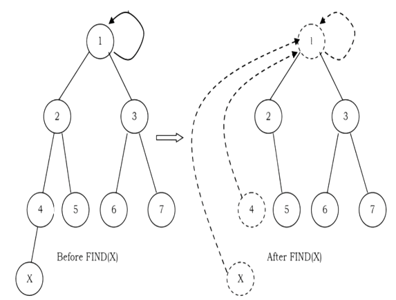
With path compression the only change to the FIND function is that S[X] is made equal to the value returned by FIND. That means, after the root of the set is found recursively, X is made to point directly to it. This happen recursively to every node on the path to the root.
FIND with path compression
void UNIONByHeight(int S[], int size, int root1, int root2){ if((FIND(S, size, root 1) == FIND(S, size, root2)) && FIND(S, size, root1) != -1)
return;
if( S[root2] < S[root])
S[root]] = root2;
else{
if( S[root2] == S[root1]){ S[root]--;
S[root2] = root];
Note: Path compression is compatible with UNION by size but not with UNION by height as there is no efficient way to change the height of the tree.
8.10 Summary
Performing m union-find operations on a set of n objects.

8.11 Disjoint Sets: Problems & Solutions
PROBLEM 1: Consider a list of cities c1; c2 ,…,cn . Assume that we have a relation R such that, for any i,j, R(ci ,cj ) is 1 if cities ci and cj are in the same state, and 0 otherwise. If R is stored as a table, how much space does it require?
Solution: R must have an entry for every pair of cities. There are Θ(n 2 ) of these.
Problem-2 For Problem-1, using a Disjoint sets ADT, give an algorithm that puts each city in a set such that ci and cj are in the same set if and only if they are in the same state.
Solution:
for (i = 1; i<= n; i++){ MAKESET(); for(j=1;j<= -1; j++){ if(R(c, c)){ UNION(cj, ci);
}
break;
Problem-3 For Problem-1, when the cities are stored in the Disjoint sets ADT, if we are given two cities ci and cj , how do we check if they are in the same state?
Solution: Cities ci and cj are in the same state if and only if FIND(ci ) = FIND(cj ).
Problem-4 For Problem-1, if we use linked-lists with UNION by size to implement the union-find ADT, how much space do we use to store the cities?
Solution: There is one node per city, so the space is Θ(n).
Problem-5 For Problem-1, if we use trees with UNION by rank, what is the worst-case running time of the algorithm from Problem-2?
Solution: Whenever we do a UNION in the algorithm from Problem-2, the second argument is a tree of size 1. Therefore, all trees have height 1, so each union takes time O(1). The worst-case running time is then Θ(n 2 ).
Problem-6 If we use trees without union-by-rank, what is the worst-case running time of the algorithm from Problem-2? Are there more worst-case scenarios thanProblem-5?
Solution: Because of the special case of the unions, union-by-rank does not make a difference for our algorithm. Hence, everything is the same as in Problem-5.
Problem 7 : With the quick-union algorithm we know that a sequence of n operations (unions and finds) can take slightly more than linear time in the worst case. Explain why if all the finds are done before all the unions, a sequence of n operations is guaranteed to take O(n) time.
Solution: If the find operations are performed first, then the find operations take O(1) time each because every item is the root of its own tree. No item has a parent, so finding the set an item is in takes a fixed number of operations. Union operations always take O(1) time. Hence, a sequence of n operations with all the finds before the unions takes O(n) time.
Problem-8 With reference to Problem-7, explain why if all the unions are done before all the finds, a sequence of n operations is guaranteed to take O(n) time.
Solution: This problem requires amortized analysis. Find operations can be expensive, but this expensive find operation is balanced out by lots of cheap union operations.
The accounting is as follows. Union operations always take O(1) time, so let’s say they have an actual cost of 1. Assign each union operation an amortized cost of √2, so every union operation puts 1 in the account. Each union operation creates a new child. (Some node that was not a child of any other node before is a child now.) When all the union operations are done, there is $1 in the account for every child, or in other words, for every node with a depth of one or greater. Let’s say that a find(u) operation costs 1 if u is a root. For any other node, the find operation costs an additional 1 for each parent pointer the find operation traverses. So the actual cost is (1 + d), where d is the depth of u. Assign each find operation an amortized cost of √2. This covers the case where u is a root or a child of a root. For each additional parent pointer traversed, 1 is withdrawn from the account to pay for it.
Fortunately, path compression changes the parent pointers of all the nodes we pay 1 to traverse, so these nodes become children of the root. All of the traversed nodes whose depths are √2 or greater move up, so their depths are now 1. We will never have to pay to traverse these nodes again. Say that a node is a grandchild if its depth is √2 or greater
Every time find(u) visits a grandchild, 1 is withdrawn from the account, but the grandchild is no longer a grandchild. So the maximum number of dollars that can ever be withdrawn from the account is the number of grandchildren. But we initially put $1 in the bank for every child, and every grandchild is a child, so the bank balance will never drop below zero. Therefore, the amortization works out. Union and find operations both have amortized costs of √2, so any sequence of n operations where all the unions are done first takes O(n) time.