36% off Learn to code by doing. Try hands-on Interview Preparation with Codepect PRO. Claim Discount Now
INTRODUCTION
CHAPTER
1
The objective of this chapter is to explain the importance of the analysis of algorithms, their notations, relationships and solving as many problems as possible. Let us first focus on understanding the basic elements of algorithms, the importance of algorithm analysis, and then slowly move toward the other topics as mentioned above. After completing this chapter, you should be able to find the complexity of any given algorithm (especially recursive functions).
1.1 Variables
Before going to the definition of variables, let us relate them to old mathematical equations. All of us have solved many mathematical equations since childhood. As an example, consider the below equation:
We don’t have to worry about the use of this equation. The important thing that we need to understand is that the equation has names (x and y), which hold values (data). That means the names (x and y) are placeholders for representing data. Similarly, in computer science programming we need something for holding data, and variables is the way to do that.
1.2 Data Types
The Type Of Data That a Variable Can Store are called Data Types .In the above-mentioned equation, the variables x and y can take any values such as integral numbers (10, 20), real numbers (0.23, 5.5), or just 0 and 1. To solve the equation, we need to relate them to the kind of values they can take, and data type is the name used in computer science programming for this purpose. A data type in a programming language is a set of data with predefined values. Examples of data types are: integer, floating point, unit number, character, string, etc.
Computer memory is all filled with zeros and ones. If we have a problem and we want to code it, it’s very difficult to provide the solution in terms of zeros and ones. To help users, programming languages and compilers provide us with data types. For example, integer takes 2 bytes (actual value depends on compiler), float takes 4 bytes, etc. This says that in memory we are combining 2 bytes (16 bits) and calling it an integer. Similarly, combining 4 bytes (32 bits) and calling it a float. A data type reduces the coding effort. At the top level, there are two types of data types:
• System-defined data types (also called Primitive data types)
• User-defined data types
System-defined data types(primitive data type)
Data types that are defined by system are called primitive data types. The primitive data types provided by many programming languages are: int, float, char, double, bool, etc. The number of bits allocated for each primitive data type depends on the programming languages, the compiler and the operating system. For the same primitive data type, different languages may use different sizes. Depending on the size of the data types, the total available values (domain) will also change.
For example, “int” may take 2 bytes or 4 bytes. If it takes 2 bytes (16 bits), then the total possible
values are minus 32,768 to plus 32,767 (-2
15
to 2
15
-1). If it takes 4 bytes (32 bits), then the
possible values are between -2,147,483,648 and +2,147,483,647 (-231to 231-1). The same is the
case with other data types.
User defined data types
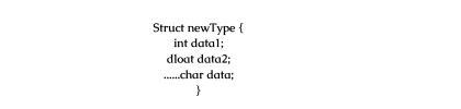
If the system-defined data types are not enough, then most programming languages allow the users to define their own data types, called user – defined data types. Good examples of user defined data types are: structures in C/C + + and classes in Java. For example, in the snippet below, we are combining many system-defined data types and calling the user defined data type by the name “newType”. This gives more flexibility and comfort in dealing with computer memory
1.3 Data Structures
Data Structure may be defined as the process of storing and organising the data with the various operations.Based on the discussion above, once we have data in variables, we need some mechanism for manipulating that data to solve problems. Data structure is a particular way of storing and organizing data in a computer so that it can be used efficiently. A data structure is a special format for organizing and storing data. General data structure types include arrays, files, linked lists, stacks, queues, trees, graphs and so on.
Depending on the organization of the elements, data structures are classified into two types:
1) Linear data structures: Elements are accessed in a sequential order but it is not
compulsory to store all elements sequentially. Examples: Linked Lists, Stacks and
Queues.
2) Non – linear data structures: Elements of this data structure are stored/accessed in a
non-linear order. Examples: Trees and graphs.
1.4 Abstract Data Types (ADTs)
Before defining abstract data types, let us consider the different view of system-defined data types. We all know that, by default, all primitive data types (int, float, etc.) support basic operations such as addition and subtraction. The system provides the implementations for the primitive data types. For user-defined data types we also need to define operations. The implementation for these operations can be done when we want to actually use them. That means, in general, user defined data types are defined along with their operations.
To simplify the process of solving problems, we combine the data structures with their operations
and we call this Abstract Data Types (ADTs). An ADT consists of two parts:
1. Declaration of data
2. Declaration of operations
Commonly used ADTs include: Linked Lists, Stacks, Queues, Priority Queues, Binary Trees, Dictionaries, Disjoint Sets (Union and Find), Hash Tables, Graphs, and many others. For example, stack uses LIFO (Last-In-First-Out) mechanism while storing the data in data structures. The last element inserted into the stack is the first element that gets deleted. Common operations of it are: creating the stack, pushing an element onto the stack, popping an element from stack, finding the current top of the stack, finding number of elements in the stack, etc.
While defining the ADTs do not worry about the implementation details. They come into the picture only when we want to use them. Different kinds of ADTs are suited to different kinds of applications, and some are highly specialized to specific tasks. By the end of this book, we will go through many of them and you will be in a position to relate the data structures to the kind of problems they solve.
1.5 What is an Algorithm?
Let us consider the problem of preparing an omelette. To prepare an omelette, we follow the steps given below:
1) Get the frying pan.
2) Get the oil.
a. Do we have oil?
i. If yes, put it in the pan.
ii. If no, do we want to buy oil?
1. If yes, then go out and buy.
2. If no, we can terminate.
3) Turn on the stove, etc…
What we are doing is, for a given problem (preparing an omelette), we are providing a step-bystep procedure for solving it. The formal definition of an algorithm can be stated as:
An algorithm is the step-by-step unambiguous instructions to solve a given problem
In the traditional study of algorithms, there are two main criteria for judging the merits of algorithms: correctness (does the algorithm give solution to the problem in a finite number of steps?) and efficiency (how much resources (in terms of memory and time) does it take to execute the).
Note: We do not have to prove each step of the algorithm
1.6 Why the Analysis of Algorithms?
To go from city “A” to city “B”, there can be many ways of accomplishing this: by flight, by bus, by train and also by bicycle. Depending on the availability and convenience, we choose the one that suits us. Similarly, in computer science, multiple algorithms are available for solving the same problem (for example, a sorting problem has many algorithms, like insertion sort, selection sort, quick sort and many more). Algorithm analysis helps us to determine which algorithm is most efficient in terms of time and space consumed.
1.7 Goal of the Analysis of Algorithms
The goal of the analysis of algorithms is to compare algorithms (or solutions) mainly in terms of
running time but also in terms of other factors (e.g., memory, developer effort, etc.)
1.8 What is Running Time Analysis?
It is the process of determining how processing time increases as the size of the problem (input size) increases. Input size is the number of elements in the input, and depending on the problem type, the input may be of different types. The following are the common types of inputs.
Size of an array
• Polynomial degree
• Number of elements in a matrix
• Number of bits in the binary representation of the input
• Vertices and edges in a graph.
1.9 How to Compare Algorithms
To compare algorithms, let us define a few objective measures:
Execution times? Not a good measure as execution times are specific to a particular computer.
Number of statements executed? Not a good measure, since the number of statements varies
with the programming language as well as the style of the individual programmer.
Ideal solution? Let us assume that we express the running time of a given algorithm as a function
of the input size n (i.e., f(n)) and compare these different functions corresponding to running
times. This kind of comparison is independent of machine time, programming style, etc.
1.10 What is Rate of Growth?
The rate at which the running time increases as a function of input is called rate of growth. Let us assume that you go to a shop to buy a car and a bicycle. If your friend sees you there and asks what you are buying, then in general you say buying a car. This is because the cost of the car is high compared to the cost of the bicycle (approximating the cost of the bicycle to the cost of the car).
Total Cost=Cost of car +Cost of Bicycle
Total Cost=Cost of car(approx)
For the above-mentioned example, we can represent the cost of the car and the cost of the bicycle in terms of function, and for a given function ignore the low order terms that are relatively insignificant (for large value of input size, n). As an example, in the case below, n 4 , 2n 2 , 100n and 500 are the individual costs of some function and approximate to n 4 since n 4 is the highest rate of growth.
n^4+2n^2+100n==n^4
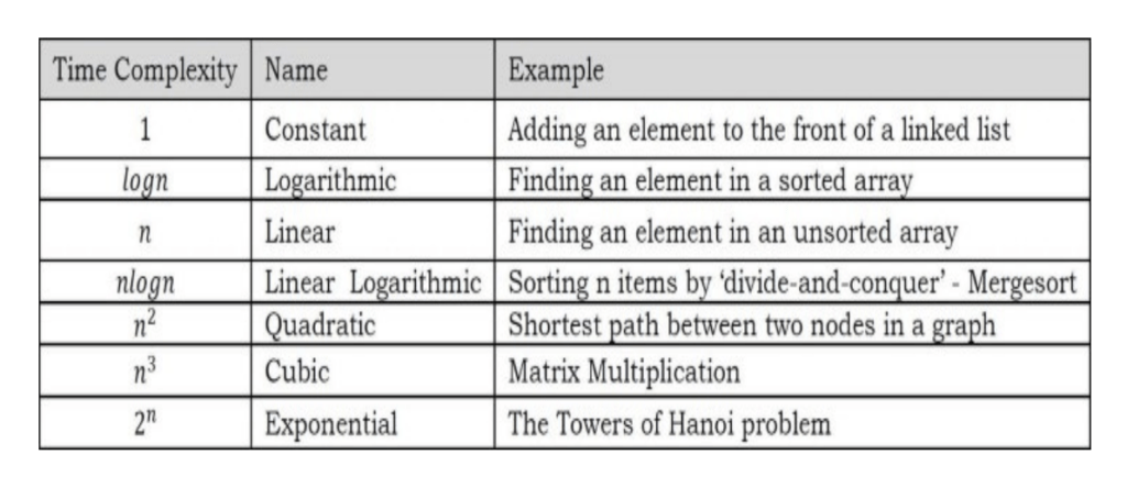
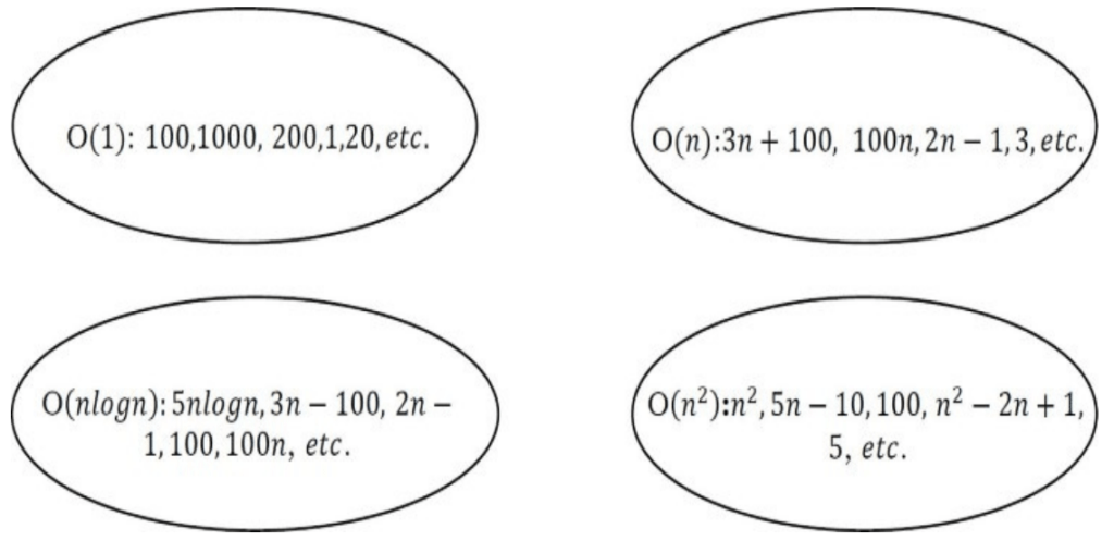
1.11 Commonly Used Rates of Growth
The diagram below shows the relationship between different rates of growth.
Highest Rate Of Growth
Rate of Growth is highest after First one
Rate of Growth is highest after Second one
Rate of Growth is highest after Third one
Rate of Growth is highest after Fourth one
Rate of Growth is highest after Fifth one
Rate of Growth is highest after Sixth one
Rate of Growth is highest after Seventh one
Rate of Growth is highest after Eight one
Rate of Growth is highest after Ninth one
Rate of Growth is highest after Tenth one
Rate of Growth is highest after 11th one
Lowest Rate of Growth
1.12 Types of Analysis
To analyze the given algorithm, we need to know with which inputs the algorithm takes less time (performing wel1) and with which inputs the algorithm takes a long time. We have already seen that an algorithm can be represented in the form of an expression. That means we represent the algorithm with multiple expressions: one for the case where it takes less time and another for the case where it takes more time.
In general, the first case is called the best case and the second case is called the worst case for
the algorithm. To analyze an algorithm we need some kind of syntax, and that forms the base for
asymptotic analysis/notation. There are three types of analysis:
Worst case
○ Defines the input for which the algorithm takes a long time (slowest
time to complete).
○ Input is the one for which the algorithm runs the slowest.
• Best case
○ Defines the input for which the algorithm takes the least time (fastest
time to complete).
○ Input is the one for which the algorithm runs the fastest.
• Average case
○ Provides a prediction about the running time of the algorithm.
○ Run the algorithm many times, using many different inputs that come
from some distribution that generates these inputs, compute the total
running time (by adding the individual times), and divide by the
number of trials.
○ Assumes that the input is random.
Lower Bound <= Average Time <= Upper Bound
For a given algorithm, we can represent the best, worst and average cases in the form of
expressions. As an example, let f(n) be the function which represents the given algorithm.
f(n)=n^2+500 for worst case
f(n)=n^2+100n+500 for best case
Similarly for the average case. The expression defines the inputs with which the algorithm takes
the average running time (or memory)
1.13 Asymptotic Notation
Having the expressions for the best, average and worst cases, for all three cases we need to identify the upper and lower bounds. To represent these upper and lower bounds, we need some kind of syntax, and that is the subject of the following discussion. Let us assume that the given algorithm is represented in the form of function f(n).
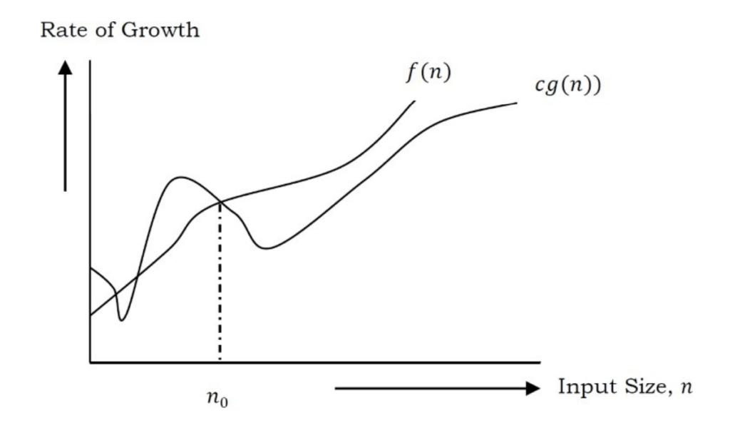
1.14 Big-O Notation [Upper Bounding Function]
This notation gives the tight upper bound of the given function. Generally, it is represented as f(n)
= O(g(n)). That means, at larger values of n, the upper bound of f(n) is g(n). For example, if f(n)
= n4 + 100n2 + 10n + 50 is the given algorithm, then n4
is g(n). That means g(n) gives the
maximum rate of growth for f(n) at larger values of n.
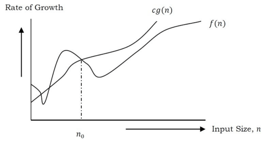
Let us see the O–notation with a little more detail. O–notation defined as O(g(n)) = {f(n): there exist positive constants c and n0 such that 0 ≤ f(n) ≤ cg(n) for all n > n0}. g(n) is an asymptotic tight upper bound for f(n). Our objective is to give the smallest rate of growth g(n) which is greater than or equal to the given algorithms’ rate of growth /(n).
Generally we discard lower values of n. That means the rate of growth at lower values of n is not important. In the figure, n0 is the point from which we need to consider the rate of growth for a given algorithm. Below n0 , the rate of growth could be different. n0 is called threshold for the given function.
Big-O Visualization
O(g(n)) is the set of functions with smaller or the same order of growth as g(n). For example;
O(n2) includes O(1), O(n), O(nlogn), etc.
Note: Analyze the algorithms at larger values of n only. What this means is, below n0 we do not
care about the rate of growth.
Big-O Examples
1.15 Omega-Q Notation [Lower Bounding Function]
Similar to the O discussion, this notation gives the tighter lower bound of the given algorithm and we represent it as f(n) = Ω(g(n)). That means, at larger values of n, the tighter lower bound of f(n) is g(n). For example, if f(n) = 100n 2 + 10n + 50, g(n) is Ω(n 2 ).
The Ω notation can be defined as Ω(g(n)) = {f(n): there exist positive constants c and n0 such that 0 ≤ cg(n) ≤ f(n) for all n ≥ n0}. g(n) is an asymptotic tight lower bound for f(n). Our objective is to give the largest rate of growth g(n) which is less than or equal to the given algorithm’s rate of growth f(n).
Ω Examples
1.16 Theta-Θ Notation [Order Function]
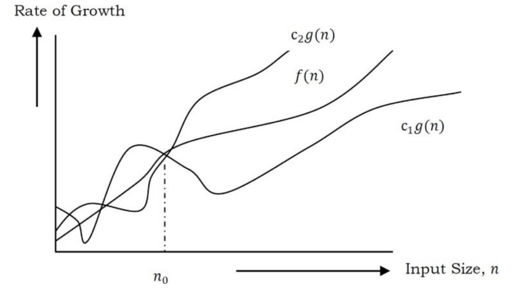
This notation decides whether the upper and lower bounds of a given function (algorithm) are the same. The average running time of an algorithm is always between the lower bound and the upper bound. If the upper bound (O) and lower bound (Ω) give the same result, then the Θ notation will also have the same rate of growth.
As an example, let us assume that f(n) = 10n + n is the expression. Then, its tight upper bound
g(n) is O(n). The rate of growth in the best case is g(n) = O(n).
In this case, the rates of growth in the best case and worst case are the same. As a result, the average case will also be the same. For a given function (algorithm), if the rates of growth (bounds) for O and Ω are not the same, then the rate of growth for the Θ case may not be the same. In this case, we need to consider all possible time complexities and take the average of those (for example, for a quick sort average case, refer to the Sorting chapter).
Now consider the definition of Θ notation. It is defined as Θ(g(n)) = {f(n): there exist positive constants c1 ,c2 and n0 such that 0 ≤ c1g(n) ≤ f(n) ≤ c2g(n) for all n ≥ n0}. g(n) is an asymptotic tight bound for f(n). Θ(g(n)) is the set of functions with the same order of growth as g(n).
Θ Examples
1.17 Important Notes
For analysis (best case, worst case and average), we try to give the upper bound (O) and lower bound (Ω) and average running time (Θ). From the above examples, it should also be clear that, for a given function (algorithm), getting the upper bound (O) and lower bound (Ω) and average running time (Θ) may not always be possible. For example, if we are discussing the best case of an algorithm, we try to give the upper bound (O) and lower bound (Ω) and average running time (Θ).
In the remaining chapters, we generally focus on the upper bound (O) because knowing the lower
bound (Ω) of an algorithm is of no practical importance, and we use the Θ notation if the upper
bound (O) and lower bound (Ω) are the same.
1.18 Why is it called Asymptotic Analysis?
From the discussion above (for all three notations: worst case, best case, and average case), we can easily understand that, in every case for a given function f(n) we are trying to find another function g(n) which approximates f(n) at higher values of n. That means g(n) is also a curve which approximates f(n) at higher values of n.
In mathematics we call such a curve an asymptotic curve. In other terms, g(n) is the asymptotic
curve for f(n). For this reason, we call algorithm analysis asymptotic analysis.
1.19 Guidelines for Asymptotic Analysis
From the discussion above (for all three notations: worst case, best case, and average case), we can easily understand that, in every case for a given function f(n) we are trying to find another function g(n) which approximates f(n) at higher values of n. That means g(n) is also a curve which approximates f(n) at higher values of n.
* There are some general rules to help us determine the running time of an algorithm.
1.20 Simplyfying properties of asymptotic notations
Transitivity: f(n) = Θ(g(n)) and g(n) = Θ(h(n)) ⇒ f(n) = Θ(h(n)). Valid for O and Ω
as well.
• Reflexivity: f(n) = Θ(f(n)). Valid for O and Ω.
• Symmetry: f(n) = Θ(g(n)) if and only if g(n) = Θ(f(n)).
• Transpose symmetry: f(n) = O(g(n)) if and only if g(n) = Ω(f(n)).
• If f(n) is in O(kg(n)) for any constant k > 0, then f(n) is in O(g(n)).
• If f1(n) is in O(g1(n)) andf2(n) is inO(g2(n)),then(f1f2(n) is inO(max(g1(n)),(g1(n))).
• If f1(n) is in O(g1(n)) and f2(n) is in O(g2(n)) then f1(n)f2(n) is in O(g1(n) g1(n)).
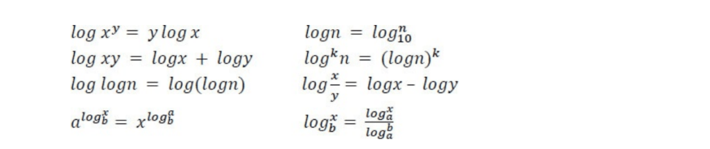
1.21 Commonly used Logarithms and Summations
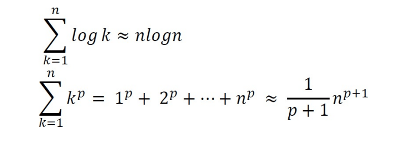
Logarithms
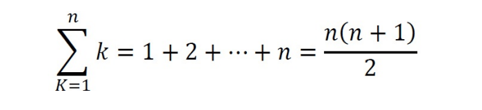
Arithmetic series
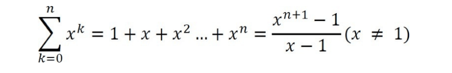
Geometric series
Harmonic series
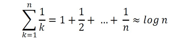
Other important formulae
1.22 Master Theorem for Divide and Conquer Recurrenc
All divide and conquer algorithms (also discussed in detail in the Divide and Conquer chapter) divide the problem into sub-problems, each of which is part of the original problem, and then perform some additional work to compute the final answer. As an example, a merge sort algorithm [for details, refer to Sorting chapter] operates on two sub-problems, each of which is half the size of the original, and then performs O(n) additional work for merging. This gives the running time equation:

The following theorem can be used to determine the running time of divide and conquer
algorithms. For a given program (algorithm), first we try to find the recurrence relation for the
problem. If the recurrence is of the below form then we can directly give the answer without fully
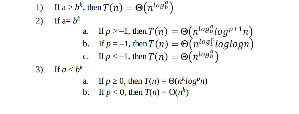
solving it. If the recurrence is of the form , where a ≥ 1,b >
1,k ≥ 0 and p is a real number, then:
1.23 Divide and Conquer Master Theorem: Problems & Solutions
For each of the following recurrences, give an expression for the runtime T(n) if the recurrence
can be solved with the Master Theorem. Otherwise, indicate that the Master Theorem does not
apply.
1.28 Algorithms Analysis: Problems & Solutions
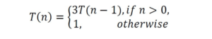 Solution: Let us try solving this function with substitution.
T(n) = 3T(n – 1)
T(n) = 3(3T(n – 2)) = 3
2T(n – 2)
T(n) = 3
2
(3T(n – 3))
.
.
T(n) = 3
nT(n – n) = 3
nT(0) = 3
n
This clearly shows that the complexity of this function is O(3
n
).
Note: We can use the Subtraction and Conquer master theorem for this problem.
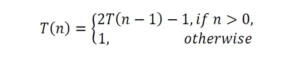 Solution: Let us try solving this function with substitution.
T(n) = 2T(n – 1) – 1
T(n) = 2(2T(n – 2) – 1) – 1 = 2
2T(n – 2) – 2 – 1
T(n) = 2
2
(2T(n – 3) – 2 – 1) – 1 = 2
3T(n – 4) – 2
2 – 2
1 – 2
0
T(n) = 2
nT(n – n) – 2
n–1 – 2
n–2 – 2
n–3
.... 2
2 – 2
1 – 2
0
T(n) =2
n – 2
n–1 – 2
n–2 – 2
n – 3
.... 2
2 – 2
1 – 2
0
T(n) =2
n – (2
n – 1) [note: 2
n–1 + 2
n–2 + ··· + 2
0 = 2
n
]
T(n) = 1
∴ Time Complexity is O(1). Note that while the recurrence relation looks exponential, the
solution to the recurrence relation here gives a different result.
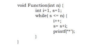 We can define the ‘s’ terms according to the relation si = si–1 + i. The value oft’ increases by 1
for each iteration. The value contained in ‘s’ at the i
th
iteration is the sum of the first ‘(‘positive
integers. If k is the total number of iterations taken by the program, then the while loop terminates
if:
P![]()
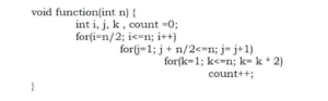 The complexity of the above function is O(n
2
logn).
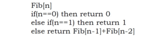 Solution: The recurrence relation for the running time of this program is: T(n) = T(n – 1) + T(n –
2) + c. Note T(n) has two recurrence calls indicating a binary tree. Each step recursively calls the
program for n reduced by 1 and 2, so the depth of the recurrence tree is O(n). The number of
leaves at depth n is 2
n since this is a full binary tree, and each leaf takes at least O(1)
computations for the constant factor. Running time is clearly exponential in n and it is O(2
n
).